tecznotes

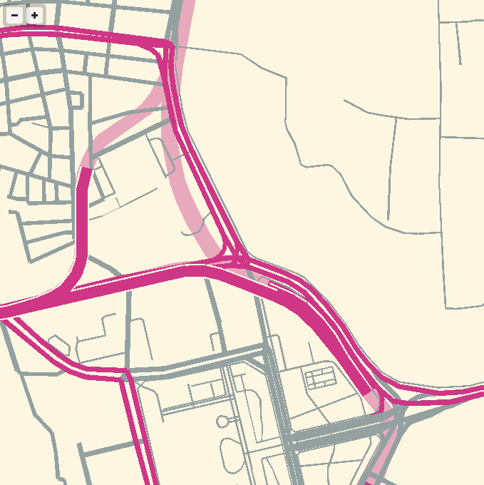
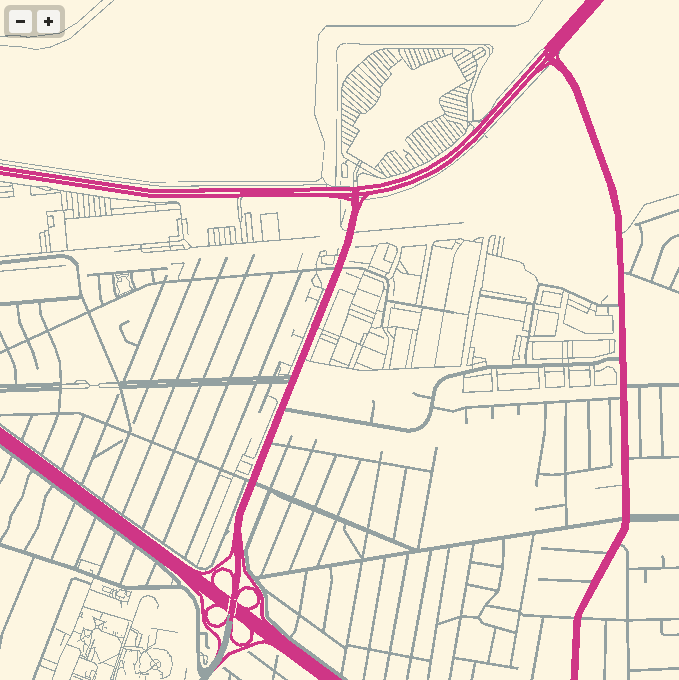
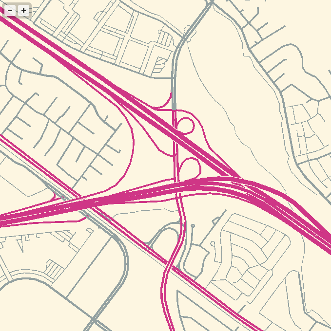
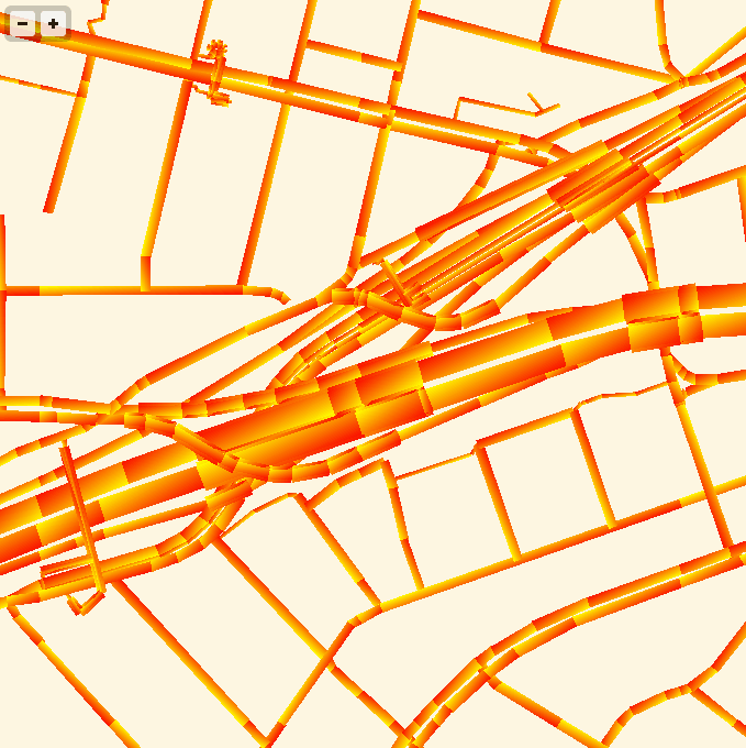
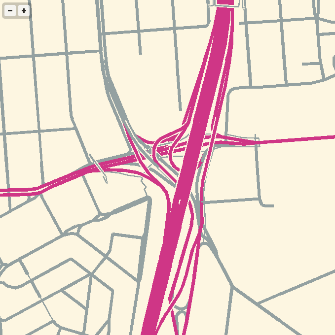
I’ve been experimenting with WebGL rendering of vector tiles from OpenStreetMap, and the results so far have been quite good.

Techniques for fast, in-browser drawing of street centerlines have interested me since I looked closely at the new iOS Google Maps, which uses vector rendering to achieve good-looking maps on the small screen of a phone.

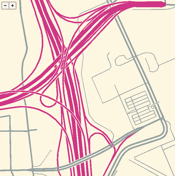
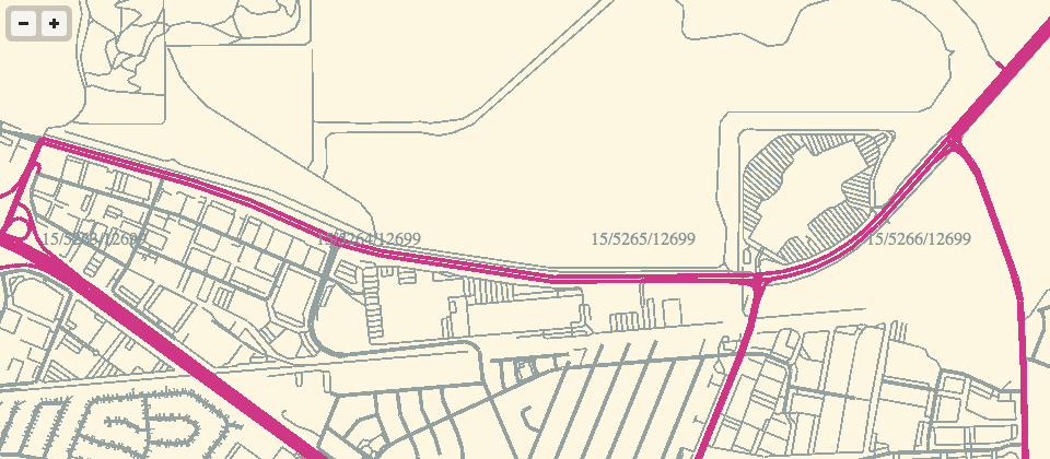
While Google seems to have aimed for an exact duplicate of their high-quality raster cartography in a more interactive package, I’ve been playing with the visual aesthetics of aliased edges and single, flat expanses of color. The jaggies along the edge of Facebook’s parking lot in the screen above remind me of early 1990s side-by-side print quality comparisons from Macworld, except I always preferred the digitally-butchered woodcut edges in the 200dpi samples to the too-perfect reproduction in the 600dpi+ version. At the very moment that they’re disappearing into a retinal haze, pixels are looking good again.

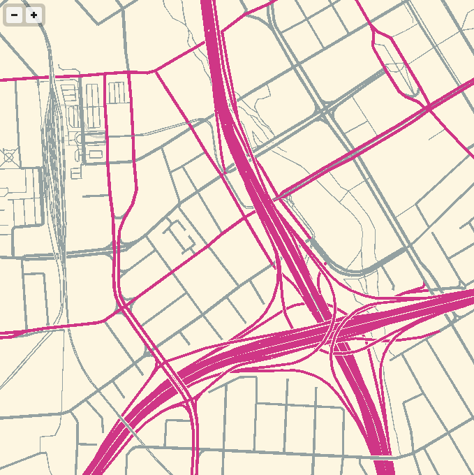
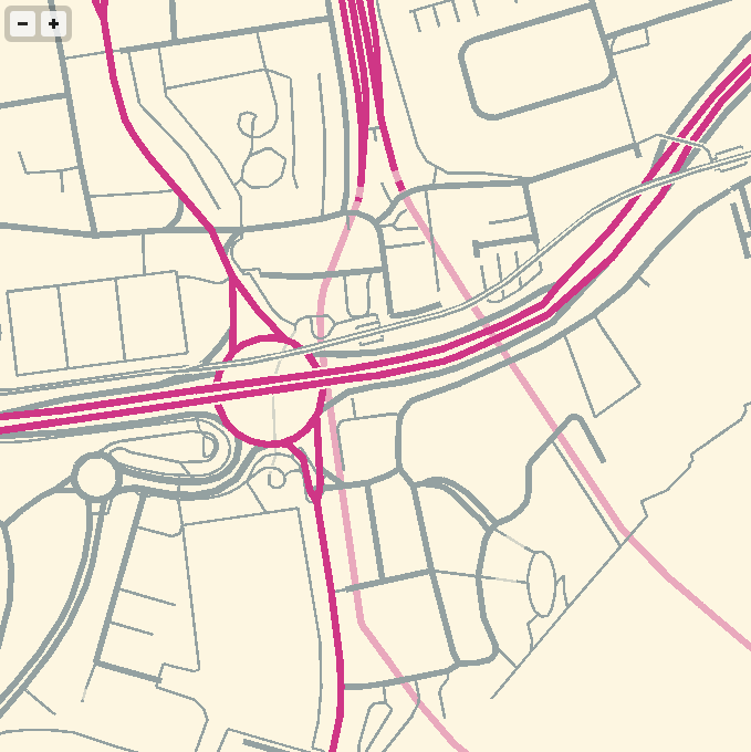
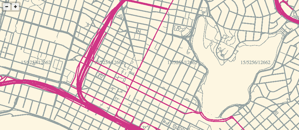
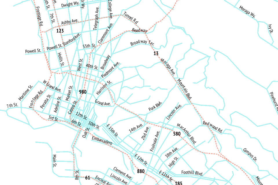
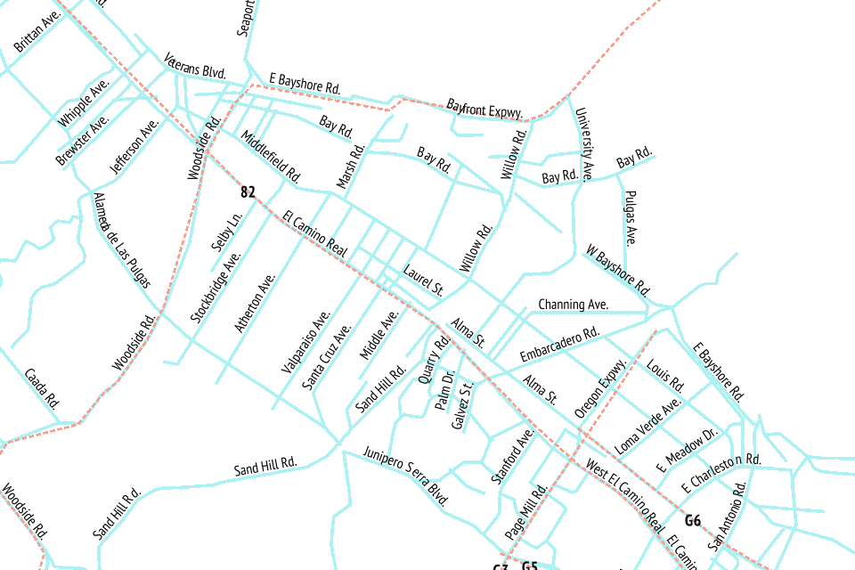
The colors here are all transposed from OSM-Solar, my cartographic application of Ethan Schoonover’s Solarized, a sixteen color palette (eight monotones, eight accent colors) designed for use with terminal and gui applications.

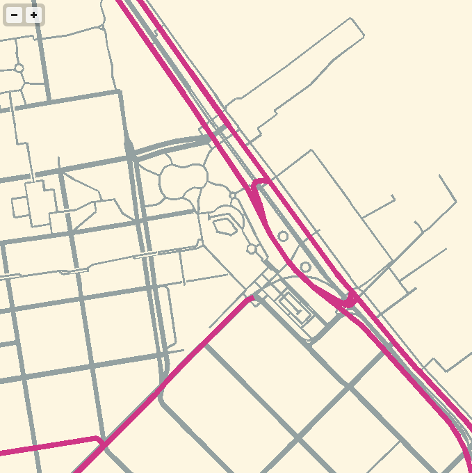
For the depth-sorting of roads and correct display of under- and overpasses, I’m using the “layer” metadata found in some OSM objects and my own High Road OSM queries. WebGL is amazing for this, because all the actual sorting is happening in the vertex shader where it can happen quickly and in parallel.

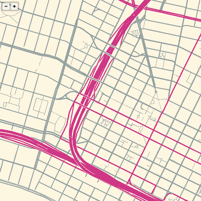
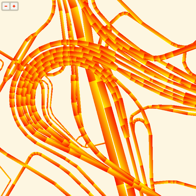
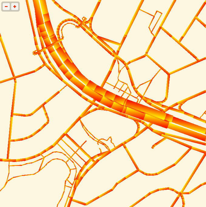
The road widths are being calculated manually, based on simplified centerline geometries found in GeoJSON tiles. I’m inflating each road type by a variable amount, manually creating my own line joins and caps. The image above is from the false color edition, which shows much more clearly how the line widths are being constructed. Javascript is reasonably fast at this basic trigonometry, but I had to move this part of the code into a web worker to cut down on animation glitches.

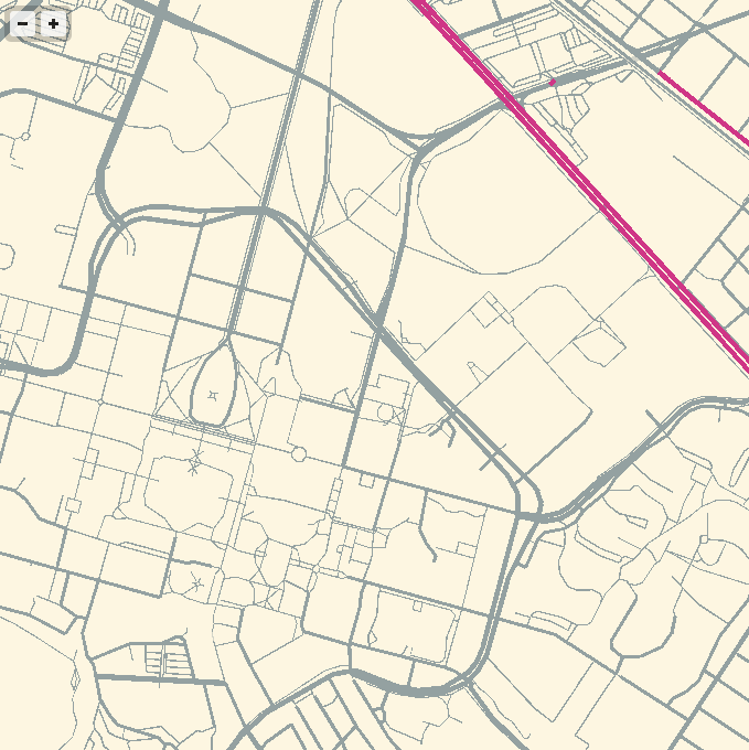
The panning and zooming smoothness are astonishing; overall I’ve been very happy with performance. One challenge that I’d like to address is the breakdown in floating point precision at zoom level 18. Four-byte floats have a 24-bit significand, which allows for pixel-perfection only up to zoom level 16 on a world map. The effect is relatively subtle at zoom 17, but glaringly obvious and a big problem at 18. I like the visual appearance of the aliased lines, but they wouldn’t be appropriate for everyday use of a map.

I imagine at some point I will need to add buildings, water and labels. One step at a time. The code for this demo is available on Github, and the correct link for the demo itself is http://teczno.com/squares/GL-Solar/.

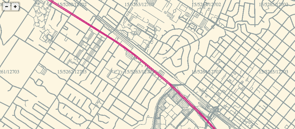
More sample screen shots below.

More about these later, but for the moment I am just loving the aliased aesthetic of pure-webGL OSM renderings.

If the color scheme looks familiar, it’s because I’ve worked with it before.

Lake Merritt is the Lenna of cartography samples. Here’s one more from Ars Technica:

—Cyrus Farivar in Ars Technica, Hands-on with RunKeeper 3 for iPhone.

Usable line generalization for OSM roads and routes has been a hobby project of mine for several years now, since I argued for it at the first U.S. State of the Map conference in Atlanta, 2010. I’ve finally put the last piece of this project in place with the use of Hadoop to parallelize the geometry processing.

I’ve learned a lot about moving geographic data between Postgres and Hadoop. The result is available at Streets and Routes.

Matt Biddulph gave me a brief introduction to using Hadoop’s streaming utility, the summary of which was that it’s just a reasonably-smart manager of scripts that push text at each other:

The utility allows you to create and run Map/Reduce jobs with any executable or script as the mapper and/or the reducer. …both the mapper and the reducer are executables that read the input from stdin (line by line) and emit the output to stdout. The utility will create a Map/Reduce job, submit the job to an appropriate cluster, and monitor the progress of the job until it completes.

(MapReduce is Google’s 2004 data processing approach for big clusters)

I’d been building something like it myself, so it was a relief to dump everything and switch to Hadoop. Amazon’s Hadoop distribution, known as Elastic MapReduce, offers an additional layer of management, handling the setup and teardown of machines for you. Communication generally happens via S3, where you load your data and scripts and pick up your results. On the EC2 side, Amazon tends to use recent versions of Debian Linux 6.0, which means that all the nice geospatial packages you’d expect from apt are available.

Easy.

For this project, I’ve added Hadoop scripts directly to Skeletron, my line-generalization tool. There’s a mapper and a reducer. Everything speaks GeoJSON because it’s easy to parse in Python and use with Shapely. If you’re familiar with pipes in Unix, the entire process is exactly equivalent to this, spread out over many machines:

cat input | mapper | sort | reducer > output

The only tricky part is in the middle, because Hadoop’s sorting and distribution of the mapped output expects single lines of text with a tab-delimited key at the beginning. In Skeletron, I created a pair of functions that convert geographic features to text (base64-encoded Well-Known Binary) and back. Only the mapper’s input and reducer’s output need to speak and understand GeoJSON. Hadoop is pretty smart about the data it reads, as well. If you tell it to look in a directory on S3 for input and it finds a bunch of objects whose names end with “.bz2,” it will transparently decompress those for you before streaming them to a mapper.

So, the process of moving data from a PostGIS table created by osm2pgsql through Hadoop takes five steps:

1. Dump your geographic data into GeoJSON files.
2. Compress them and upload them to a directory on S3.
3. Run a MapReduce job that accepts and outputs GeoJSON data.
4. Wait.
5. Pick up resulting GeoJSON from another S3 directory.

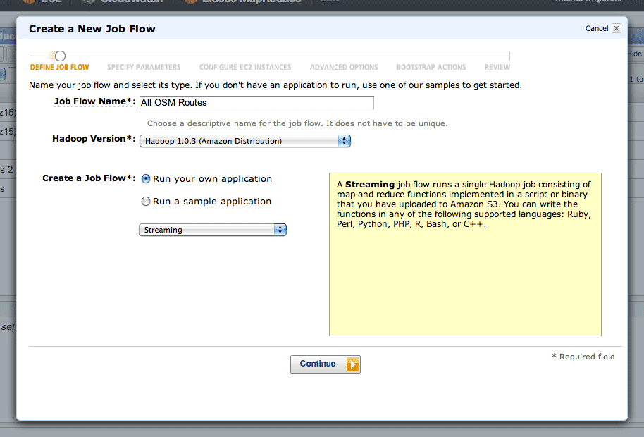
Running a MapReduce job is mostly a point-and-click affair.

After clicking the “Create New Job Flow” button from the AWS console, select the Streaming flow:

The second step is where you define your inputs, outputs, mappers and reducers:

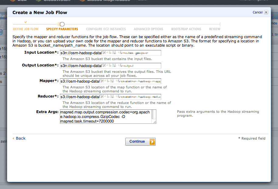
The “s3n:” protocol is used to refer to directories on S3, and the “osm-hadoop-data” part in the examples above is my bucket. For the mapper and reducer, I’ve uploaded the scripts directly from Skeletron so that EMR can find them.

The extra arguments I’ve used are:

• -D mapred.task.timeout=21600000 to give each map task six hours without Hadoop flagging it as failed. By default, Hadoop assumes that a task will take five minutes, but some of the more complex geometry tasks can take hours.
• -D mapred.compress.map.output=true to compress the data moving between the mappers and reducers, because it’s large and repetitive. The compression codec is given by -D mapred.map.output.compression.codec=org.apache.hadoop.io.compress.GzipCodec.
• -D mapred.output.compress=true to compress the output data sent to S3. The compression codec is given by -D mapred.output.compression.codec=org.apache.hadoop.io.compress.BZip2Codec.

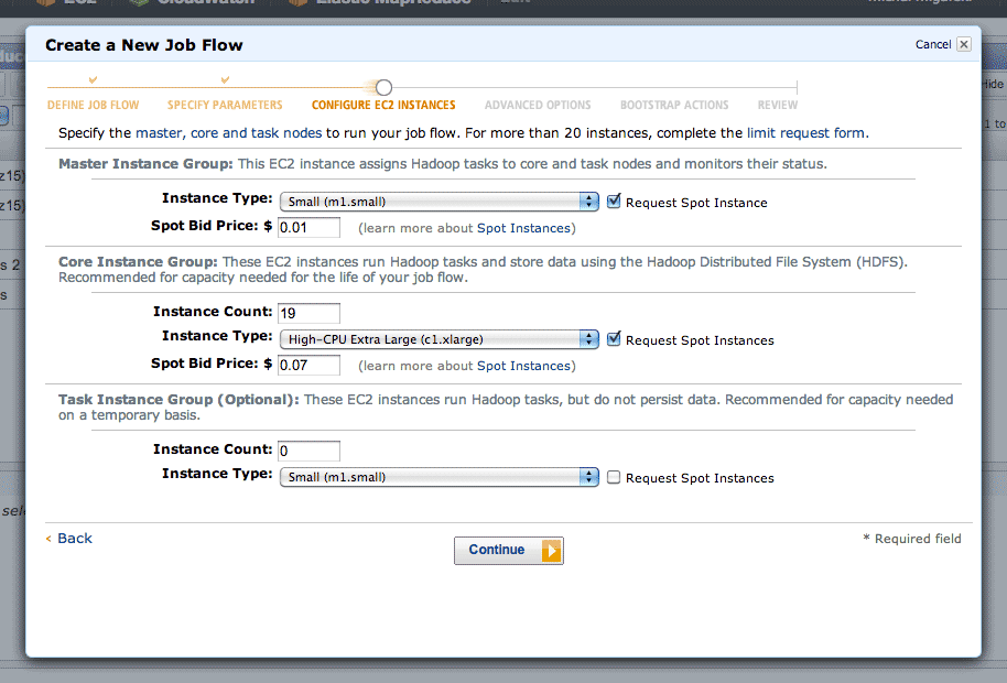
Step three is where you choose your EC2 machines. Amazon’s spot pricing is a smart thing to use here. I’ve typically seen prices on the order of $0.01 per CPU-hour, a huge savings on EC2’s normal pricing. Using the spot market will introduce some lag time to your job, since Amazon assumes you are a flexible cheapskate. I’ve typically experienced about ten minutes from creating a job to seeing it run.

In step four, there are two interesting advanced options. Setting a log path will get you a directory full of detailed job logs, useful when something is mysteriously failing. Setting a key pair will allow you to SSH into your master instance, which runs a detailed Hadoop job tracker UI over HTTP on port 9100 (SSH tunnel in to see it in a browser). The tracker lets you dig into individual tasks or see an overall progress graph.

Step five is where you can define a setup script. This script is where you’ll do all of your per-machine preparation, such as downloading uniform data or installing additional packages.

For lengthy jobs, EMR’s graphs are a useful way to observe job flow progress. Your two most useful graphs are Average Map Tasks Running (top left), telling you how many mapper tasks are currently in progress, and Average Map Tasks Remaining (second from left on the top row), telling you how many mapper tasks have not yet started.

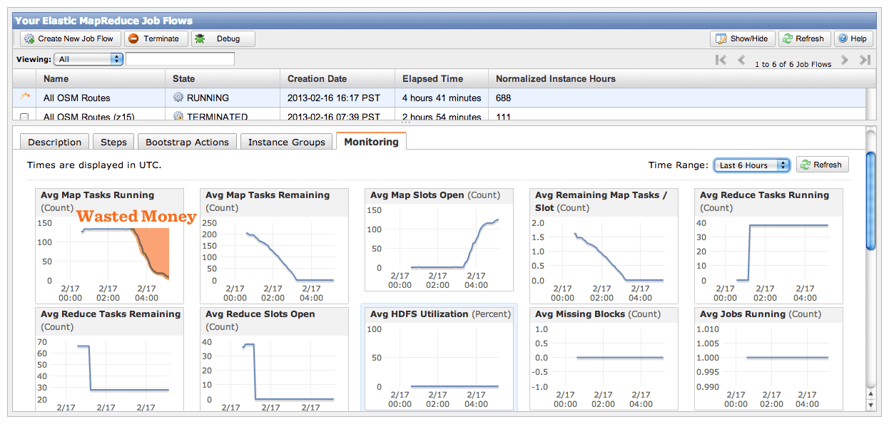
While the job is in progress, you’ll see the second graph progress downward toward zero, and the first graph pegged to the top and then progressing downward as well. The amount of time the first graph spends below the maximum represents wasted money, spent on CPU’s twiddling their thumbs waiting for straggler jobs to come in. This problem will be worse if you have more machines working on your job, leading to a very simple speed/cost tradeoff. If you want your job done fast, some of your machines won’t be doing much once the main crush is over. If you want your job done cheap, keep a smaller number of machines going to reduce the number of idle processors at the end.

I ran the same job twice with a different number of machines each time, and saw a cost of $4.90 for five instances over 17 hours vs. $9.40 for twenty instances over 7 hours. If you don’t need the results fast, save the five bucks and let it run overnight. If you don’t use spot pricing, this same job would have cost $40 slow or $78 fast.

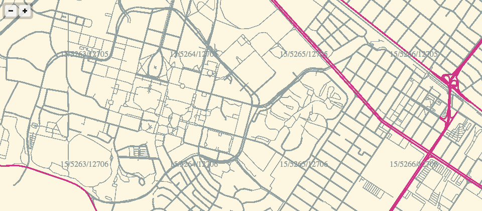
To try all this yourself, I’ve set up a bucket with sample data from the OSM route relations job.

The end result is something I’m super happy about: a complete worldwide dataset of simplified roads and routes that’s suitable for high-quality labels and route shields.

We saw Beasts of the Southern Wild yesterday, still thinking about it today. It’s a beautiful, surrealist, magical realist story about a hurricane evacuation south of New Orleans. Everything is told through the eyes of a six year old, whose acceptance of the facts of nature around shocked me, one after another. All animals are made out of meat. Prehistoric aurochs thawing from the arctic ice and floating down to the Gulf of Mexico. Streams of gorgeous, post-apocalyptic imagery. Perfect acting by Dwight Henry.

On an airplane coming back from Washington, DC. I’m trying to be good at this weeknotes thing, but I’m also somewhat speechless for the moment so this will be short.

Code is a thing I can talk about most comfortably in the context of a weeknote, otherwise it turns into strangely unsatisfying codename mystery project blogging.

I’ve formalized last week’s Typescript experiment into a standalone map tile library called Squares. A demo that loosely duplicates the recently-departed getlatlon.com shows what it’s generally capable of, which at the moment is Not A Ton. I think the Typescript experiment feels like a success, and I’m starting to point Squares at other projects that have been waiting for it to take shape.

When I wasn’t hacking at Typescript last week, I was at an actual desk working with Trifacta in San Francisco on data and UX consulting.

We also had a record nine people at our weekly geogeek breakfast at the Mission Pork Store, up from a typical five or six. Onward.

While in DC, I fully caught up with Team Mapbox and batted around some OpenStreetMap US 2013 ideas with Eric, Alex, Tom, and Bonnie. We watched Ted, the one about the talking bear, and drank cheap beer from cans.

This week, more of all that and talking and hopefully some new code and cartography finally.

This has been week six of self-exile and funemployment.

Since JS.Geo, I’ve been reflecting on the world-consuming popularity of Mike Bostock and Jason Davies’s D3 library and giving it a repeat test-drive. I think there are two fascinating aspects to the public response to D3 at events like JS.Geo: everyone wants to do something with it, but very few people claim to understand it. I attempted to explain the “.data()” method to a friend at JS.Geo and realized that I also was missing a critical piece myself. One metaphor I’ve been using to think about D3 has been performance: Mike and Jason are so deeply good at what they do and create such a prolific stream of examples that just watching the work is like a stage performance. They’re the current reigning Penn & Teller of Javascript, the Las Vegas tiger guys of SVG, and you can’t not be fascinated even as your watch disappears. The problem with this metaphor is that it puts up a wall between you and the code, frames it as an unobtainable skill. There’s not much you can learn about personal fitness from watching a professional dancer at work. So, performance is an unhelpful metaphor.

A more useful metaphor I’ve been exploring in code this week is D3 as nuclear fuel. This starts to feel a bit more helpful, because it suggests a clear approach to D3 for mortal developers: use the power, but keep it carefully contained. It’s the same line of thinking suggested by Rebecca Murphey’s argument about jQuery: “it turns out jQuery’s DOM-centric patterns are a fairly terrible way to think about applications,” leading to Tom Hughes-Croucher’s idea of pyramid code, “huge chains of nested, dependent anonymous callbacks piled one on top of another.” With great power comes great blah blah blah. Observing Dr. Manhattan offers little guidance for building a power plant.

I’ve always enjoyed strongly-typed languages for interactive work, so this week I have been approaching the use of D3 from the direction of Typescript, Microsoft’s typed superset of JavaScript that compiles to plain JavaScript. The Typescript team have helpfully created a starting set of declarations for D3, making it possible to use the relatively-structureless method chains within a more controlled environment.

I’m surprised at how much I enjoyed Typescript, and how comfortable it felt immediately, and how fun it’s been to bounce a free-form library like D3 against a strictly-typed language environment, like a super ball off a concrete wall. My test project is a fork of Tom Carden’s D3Map, an exercise in learning D3 for DOM manipulation and transitions. Play with it live at bl.ocks.org/4703593. You can use Typescript to write legible, self-describing code with clearly enforced expectations like Grid.ts. You can also keep the D3-needing parts carefully separated from the tile math like Image.ts and Mouse.ts. The additional structure demanded by Typescript felt surprising calming, like Allen Short’s 2010 PyCon talk on Big Brother’s Design Rules (via War is Peace):

• Slavery is Freedom: the more you constrain your code's behavior, the more freedom you have to act.
• Ignorance is Strength: the less your code knows about, the fewer things it can break. This is itself a play on the Law of Demeter or principle of least knowledge.

The one major bump I experienced with Typescript was in deploying to a browser. Although Typescript files compile to Javascript, they include calls to “require(),” a part of the CommonJS spec. This is not browser-kosher, so I used Browserify in the Makefile to generate a browser-compatible file with an extra 9KB slug of CommonJS overhead.

All of this has been a step on the way to a browsable WebGL map, one of my goals from last week.

I have also significantly updated the visual appearance of Green Means Go to make it more legible and hopefully printable.

No current progress on Metro Extracts.

This week, I’ll be doing some consulting and some future conspiracy planning. People will be visiting town, and I will have beers with them.